不论是目标区域测序还是外显子组测序还是全基因组测序之后，我们会关注目标区域在特定深度下的覆盖度。比如20X的比例，50X的比例。如果只计算特定深度的覆盖度，我们了解不到其他深度下的覆盖度情况。如果每个都列出来，又不直观，这个时候用图片来表示就非常直观了。

获取统计数据

我们需要知道在每个深度下碱基的比例，这个时候强大的bedtools就出场了。

bedtools coverage -sorted -hist -g genome.file  -b  samp.bam -a target_regions.bed ' grep ^all > samp.hist.all.txt

-hist是为了获取目标区域的总结信息，以all开头，输出每个每个深度下碱基的比例，所以后续用grep ^all来过滤。

-sorted可以节省内存，但需要通过-g跟genome file来指定染色体的顺序。

genome file可以通过awk -v OFS='\t' {‘print $1,$2’} genome.fa.fai > genome.file 得到。

假设我们得到了smp1.hist.all.txt、smp2.hist.all.txt、smp3.hist.all.txt、smp4.hist.all.txt、smp5.hist.all.txt、smp6.hist.all.txt、smp7.hist.all.txt、

作图

 1
 2
 3
 4
 5
 6
 7
 8
 9
10
11
12
13
14
15
16
17
18
19
20
21
22
23
24
25
26
27
28
29
30
31
32
33
34
35
36
37
38
39
40

# Get a list of the bedtools output files you'd like to read in

print(labs <- paste("", gsub(".hist.all.txt", "", files, perl=TRUE), sep=""))


# Create lists to hold coverage and cumulative coverage for each alignment,
# and read the data into these lists.
cov <- list()
cov_cumul <- list()
for (i in 1:length(files)) {
    cov[[i]] <- read.table(files[i])
    # The value should be 1 at 0X.
    cov_cumul[[i]] <- 1-cumsum(c(0,cov[[i]][,5]))
}

library(RColorBrewer)
cols <- brewer.pal(length(cov), "Dark2")

# Save the graph to a file
png("target-coverage-plots.png", h=1000, w=1000, pointsize=20)

# Create plot area, but do not plot anything. Add gridlines and axis labels.
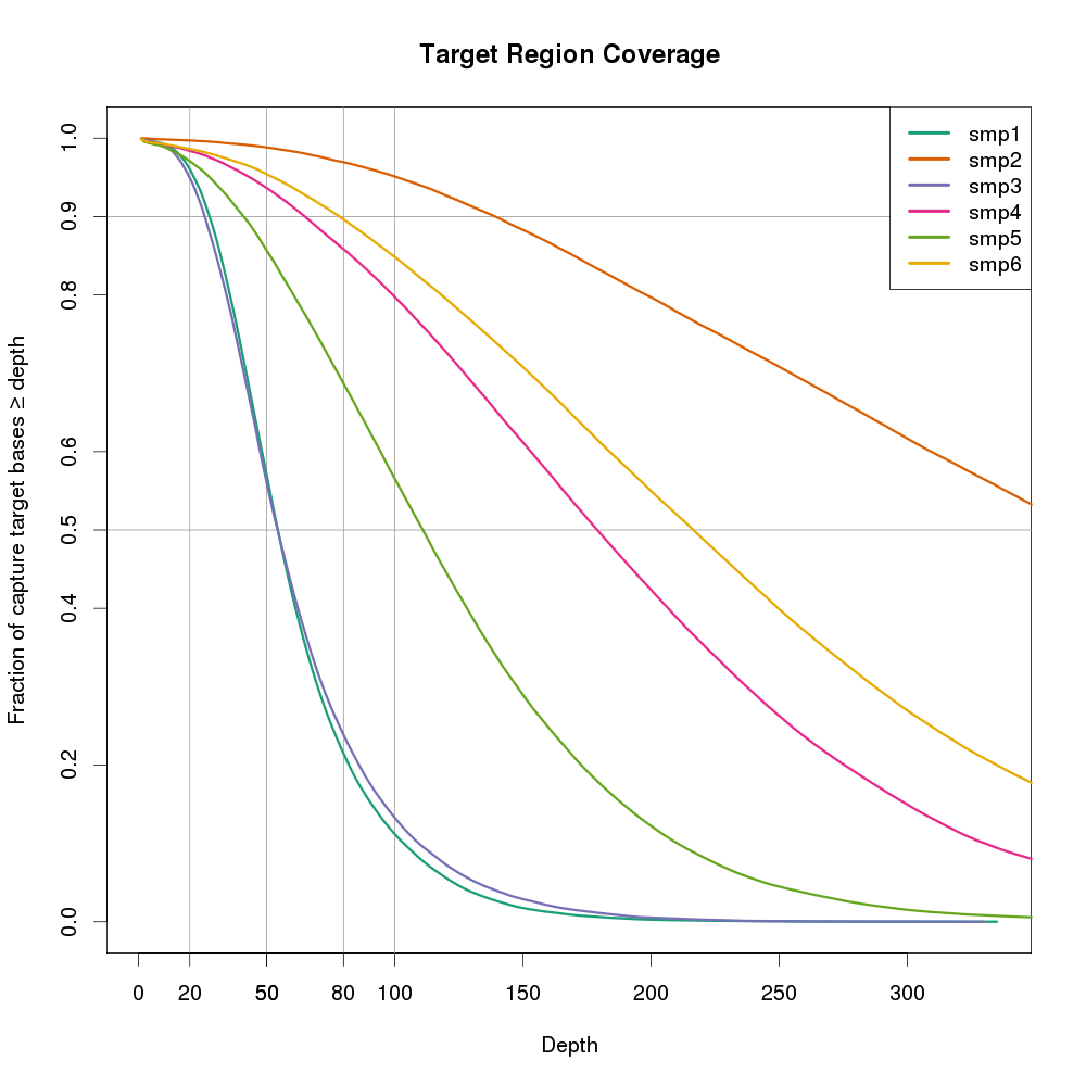
plot(cov[[1]][2:401, 2], cov_cumul[[1]][1:400], type='n', xlab="Depth", ylab="Fraction of capture target bases \u2265 depth", ylim=c(0,1.0), main="Target Region Coverage")
abline(v = 20, col = "gray60")
abline(v = 50, col = "gray60")
abline(v = 80, col = "gray60")
abline(v = 100, col = "gray60")
abline(h = 0.50, col = "gray60")
abline(h = 0.90, col = "gray60")
axis(1, at=c(20,50,80), labels=c(20,50,80))
axis(2, at=c(0.90), labels=c(0.90))
axis(2, at=c(0.50), labels=c(0.50))

# Actually plot the data for each of the alignments (stored in the lists).
for (i in 1:length(cov)) points(cov[[i]][2:401, 2], cov_cumul[[i]][1:400], type='l', lwd=3, col=cols[i])

# Add a legend using the nice sample labeles rather than the full filenames.
legend("topright", legend=labs, col=cols, lty=1, lwd=4)

dev.off()

FASTQ文件在Illumina下机数据文件夹Data\Intensities\BaseCalls**中，类似SampleName_S1_L001_R1_001.fastq.gz（比如NTC_S11_L001_R1_001.fastq.gz）**

其中被下划线_分为了五个部分。

• 第一部分：SampleName，样本名，与上机时在Sample Sheet中填写的一致

• 第二部分：S1，S***，S后跟的数字与样本在Sample Sheet中的顺序一致，从1开始。不能分配到确定样本的read会归到S0（Undetermined_S0）

• 第三部分：L00*，泳道lane的编号

• 第四部分：R*，R1表示read1，R2表示read2。R1和R2为paired end reads。同一个样本的配对的FASTQ，只有这个地方不同

• 第五部分：001，通常为001

  Naming

  FASTQ files are named with the sample name and the sample number, which is a numeric assignment based on the order that the sample is listed in the sample sheet.

  Example:

  Data\Intensities\BaseCalls\SampleName_S1_L001_R1_001.fastq.gz

  • SampleName-The sample name provided in the sample sheet. If a sample name is not provided, the file name includes the sample ID, which is a required field in the sample sheet and must be unique.

  • S1-The sample number based on the order that samples are listed in the sample sheet starting with 1. In this example, S1 indicates that this sample is the first sample listed in the sample sheet.

GATK4正式版已经发布，快去体验啦。GATK4在上一年提出开源，并放出beta版本，现在终于姗姗来迟。

GATK4是业界第一次涵盖了胚细胞和体细胞基因型分析中的主要突变类型的基因组分析工具，且已经开源。新版本的GATK为了解决性能瓶颈近乎完全重构，提高了速度和扩展性有不失其过往的准确度。

GATK4包含了备受大家喜爱的pipeline和新工具，汲取了机器学习和神经网络算法的优点。

在用Picard跑sortSam或者markDuplicate的时候，报错

RuntimeIOException: java.io.IOException: No space left on device

提示硬盘空间不足，实际上节点的硬盘空间是够的。这是因为Picard在做这两个处理的时候，会生成临时文件，临时文件默认储存在系统的tmp文件夹。这个文件夹内的文件存储一些程序和软件的临时文件，在RHEL6中，系统自动清理/tmp文件夹的默认时限是30天。可以通过/etc/cron.daily/tmpwatch配置,在Ubuntu中，系统自动清理/tmp文件夹的时限默认每次启动。而全基因组和全外显子组的数据非常大，现在分给系统的空间都很小，导致tmp文件夹写满而报错。

处理方法：

在个人home文件夹下，新建一个tmp文件夹，每次运行picard的时候，指定IO临时文件夹为这个文件夹。

1
2

mkdir $HOME/tmp
java -Xmx2g -Djava.io.tmpdir=$HOME/tmp -jar SortSam.jar SORT_ORDER=coordinate INPUT=input.bam OUTPUT=output.sort TMP_DIR=$HOME/tmp

不能使用~，picard会在工作目录下创建'~‘文件夹。

数据分析中会经常用到bed文件，有时候bed文件中的区域有重叠时会影响统计结果，或者没有按照顺序排序时会影响代码的逻辑。合并bed文件或者文件中的区域是经常进行的。

我常用的工具是bedtools的merge功能，官方示例如下：

1
2
3
4
5
6
7
8

$ cat A.bed
chr1  100  200
chr1  180  250
chr1  250  500
chr1  501  1000
$ bedtools merge -i A.bed
chr1  100  500
chr1  501  1000

bedtools的merge功能强大的地方，更在于在合并的时候，可以进行一下操作。如下操作，通过-c指定要操作的目标列，-o指定操作动作。