思考:是否升级参考基因组版本
Should I switch to a newer reference?
GRCh38 consists of several components: chromosomal assembly, unlocalized contigs (chromosome known but location unknown), unplaced contigs (chromosome unknown) and ALT contigs (long clustered variations). The combination of the first three components is called the primary assembly. It is recommended to use the complete primary assembly for all analyses.
参考基因组包括chromosomal assembly, unlocalized contigs (chromosome known but location unknown), unplaced contigs (chromosome unknown)和ALT contigs (long clustered variations),前三个是primary assembly,alt contigs代表的是部分区域单体型的多样性,这些区域过于复杂不能用一条序列表示。
In addition to adding many alternate contigs, GRCh38 corrects thousands of SNPs and indels in the GRCh37 assembly that are absent in the population and are likely sequencing artifacts. It also includes synthetic centromeric sequence and updates non-nuclear genomic sequence.
除了添加了很多alternative contigs,GRCh38更正了数以千计的GRCh37版本中的SNPs和indels,这些SNPs和indels在人群中没有出现过、可能因为测序错误导致。GRCh38版本也包含了人工的着丝粒序列和更新了非核基因组序列。
The ability to recognize alternate haplotypes for loci is a drastic improvement that GRCh38 makes possible. Going forward, expanding genomics data will help identify variants for alternate haplotypes, improve existing and add additional alternate haplotypes and give us a better accounting of alternate haplotypes within populations. We are already seeing improvements and additions in the patch releases to reference genomes, e.g. the seven minor releases of GRCh38 available at the time of this writing. GRCh38大幅提高了识别alternate haplotype的能力,进一步提高了识别alternate haplotype的突变的能力。
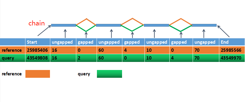
BWA的作者Li Heng推荐GRCh37 primary assembly+ALT+decoy组成的参考基因组hs38DH,可以通过bwa下载,见https://github.com/lh3/bwa/blob/master/README-alt.md :
bwa.kit/run-gen-ref hs38DH
作者的用NA12878做测试的比对结果如下,
|
|