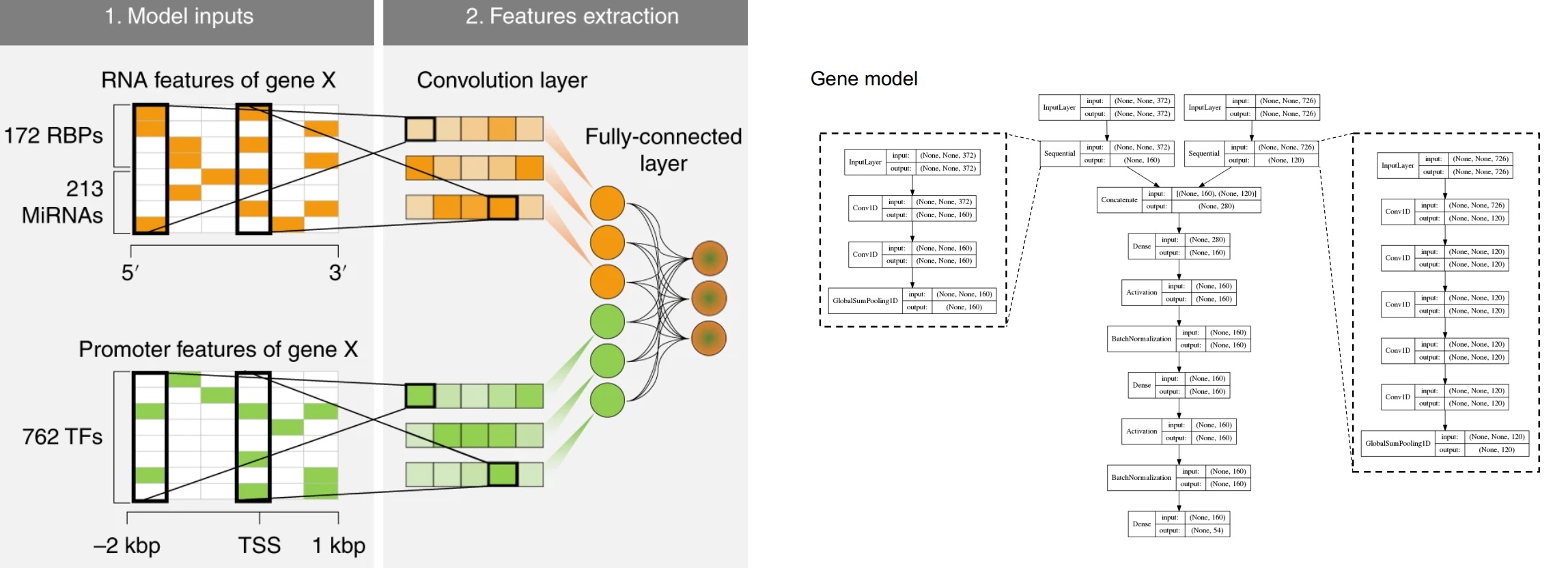
保存几张1D卷积的图和文章，方便以后查找，摘自互联网。说不准以后搞深度学呢🫠🙃卷的结果就是以后不上人工智能都不要意思说自己是搞生信的。

主要是看到一篇文章，用了卷积神经网络，我一直就好奇组学数据怎么做卷积，所以就看了下文章，发现用的是Conv1D。（不知道理解的对不对）对于1D卷积Conv1D而言，如果卷积核kernel size是2的话，最终会生成一个 “行数-kernel size+1“的向量，如果数据分批给的话，就有batch，比如如果样本是21000，batch size是128的话，每个batch有165个样本，所以Nature Machine Intelligence的附图 Fig. 10这篇文章还进行了BatchNormalization。

Samples = 21000, batch_size=128 -> training_sample for each epoch = 21000/128 = 164.06 ~= 165

https://stackoverflow.com/questions/72529761/batch-size-in-input-shape-statement-for-keras-conv1d-layers

filters可以指定多次卷积（相同kernel size），这样可以生成二维的数据。

Deep learning decodes the principles of differential gene expression

遇到的情形

分析的代码已经调试好，但分析的时间较长；

后端启动jupyter notebook后，奈何网络不稳定，notebook经常掉线，跑到一半的程序就断掉了；

服务器其他人的jupyter notebook的端口如果和我的一样，别人启动jupyter notebook后，我正在用的端口就会往后变。

于是我就想，能否在终端直接运行.ipynb文件，这样我就可以加nohup命令了，或者把ipynb的代码转成python，我nohup运行python也行。

基于以上情况，我google到了nbconvert。

nbconvert

nbconvert的github地址：https://github.com/jupyter/nbconvert

jupyter nbconvert通过模版引擎jinja将ipynb文件转成其他格式的文件，包括

• HTML
• LaTeX
• PDF
• Reveal JS
• Markdown (md)
• ReStructured Text (rst)
• executable script

此外nbconvert还有另外一个功能就是通过–execute选项在终端执行ipynb文件

安装nbconvert

1
2

pip install nbconvert
# 或者conda install nbconvert

ipynb格式转换

1
2
3
4
5

# 转成python，转成后，后有前缀和ipynb一样的py文件，运行这个就行。
jupyter nbconvert --to python --execute mynotebook.ipynb
# --to后面跟格式，比如html
jupyter nbconvert --to html mynotebook.ipynb
# 支持的格式包括['asciidoc', 'custom', 'html', 'html_ch', 'html_embed', 'html_toc', 'html_with_lenvs', 'html_with_toclenvs', 'latex', 'latex_with_lenvs', 'markdown', 'notebook', 'pdf', 'python', 'rst', 'script', 'selectLanguage', 'slides', 'slides_with_lenvs']

上面是格式转换，在转换的过程中，比如转pdf、latex的时候，可能还需要额外的包，比如pandoc等，还需要额外安装。可以参考https://nbconvert.readthedocs.io/en/latest/index.html

jupyter nbconvert还有个功能就是执行ipynb格式的文件，如下

1
2
3
4
5

jupyter nbconvert --execute mynotebook.ipynb
# 这个时候就和linux终端下的正常命令类似了，比如加上重定向
jupyter nbconvert --execute mynotebook.ipynb >> mylog.out.log 2>&1
# 还可以和格式转换相结合
jupyter nbconvert --to python --execute mynotebook.ipynb

假设我想把通过运行jupyter nbconvert执行ipynb文件的过程更简单点，可以通过在.profile里面设置命令的别名

1
2
3
4

# .profile或者.bashrc里面配置
alias nbx="jupyter nbconvert --execute"
# 终端运行ipynb文件
nbx mynotebook.ipynb

当进行Isoseq的样本测了多次，或者多个run时，可能会碰到合并subreads.bam文件。我倾向先合并再往后分析，兼容以前的流程，避免分别分析再合并会遇到其他错误。Pacbio Isoseq的下机数据格式已经从h5变成了subreads.bam，合并其实很简单，和samtools类似，但得用pacbio的工具才行，当然还要建立index生成pbi文件，也是用pacbio的工具。

1
2
3
4

# merge
pbmerge -o merged.bam data_1.bam data_2.bam data_3.bam
# index
pbindex merged.bam

VAF - variant allele frequency

Variant allele fraction or frequency (VAF): the fraction of mutated reads for a given variant, which is a readout for the proportion of DNA mutated in the sequenced tissue.

测序时特定位点突变的reads数比上总的reads数，可以从VCF中获得。

CCF - cancer cell fraction

Cancer cell fraction (CCF): the fraction of cancer cells from the sequenced sample carrying a set of SNVs.

携带突变的癌细胞比例，可以通过pyclone（https://github.com/Roth-Lab/pyclone-vi）或sciclone（https://github.com/genome/sciclone）计算。

$$ CCF = VAF *\frac{1}{p}[pCN_t + CN_n(1-p)] $$

VAF: corresponds to the variant allele frequency at the mutated base

p: the tumor purity肿瘤纯度

CNt: the tumor locus specific copy number所在位置的拷贝数

CNn: the normal locus specific copy number (CNn was assumed to be 2 for autosomal chromosomes)正常样本的拷贝数

三种时间依赖的ROC

诊断模型的ROC是大家最熟悉的，一组二分类的真实标签，一组风险分值，不同的cutoff下有不同的灵敏度和特异性，就能画出ROC曲线。

生存分析一般建立Cox模型，根据Cox模型也会有一组风险分值，生存结局也是一个二分类的标签，但病例多了时间的信息。

三种不同的定义来估计删失事件的时间依赖的敏感性和特异性，即（1）cumulative/dynamic累积/动态（C/D），（2）incident/dynamic事件/动态（I/D）和（3） incident/static事件/静态 (I/S)。不同的定义下，灵敏度和特异性的计算不一样。其中C/D比I/D和I/S更具有临床相关性，在临床中普遍使用。

t: 目标时间，t* 固定的随访时间，c 阈值，A-F为研究中的个体病例，其中ABC的指标高于c，DEF个体的指标小于c，实心圆表示发生事件的个体，空心圆表示Censored个体。

图a，C/D、I/D、I/S中的相对于基线时间点的实验和对照个体说明，图b，I/S（纵向）的说明

Cumulative sensitivity and dynamic specificity (C/D)

$$ \begin{array}{l} S{e}^C\left( c, t\right)= P\left({X}_i> c\Big|{T}_i\le t\right)\\ {} S{p}^D\left( c, t\right)= P\left({X}_i\le c\Big|{T}_i> t\right)\\ {} AU{C}^{C, D}(t)= P\left({X}_i>{X}_j\Big|{T}_i\le t,{T}_j> t\right), i\ne j.\end{array} $$

cumulative/dynamic(C/D)中cumulative是指Cumulative sensitivity，dynamic是指dynamic specificity。C/D是用的最广泛的ROC模型。

灵敏度：生存时间小于t的人群之中，Xi大于阈值c的人群（A和B个体）所占总体（A、B和E）的比例

特异度：生存时间大于t的人群之中，Xi小于等于阈值c的人群（D和F）所占总体（C，D和F）的比例

用二分类模型来类比，时间ROC，在选定特定时间点（比如1年、3年或者5年）时，不同的阈值c可以将队列人群分成高于c的一组（高风险，认为发生了死亡/事件）和小于等于c（低风险，认为没有发生死亡/事件），但这个时间点有真实的死亡或者事件的标签，于是可以计算在特定时间点特定c时的灵敏度和特异性，进行画ROC计算AUC。所以文献中经常看到1yr, 3yr, 5yr ROC的图，有了ROC的图，其实也可以画DCA进行DCA分析。