TCGABiolinks下载TCGA数据做生存分析

 1
 2
 3
 4
 5
 6
 7
 8
 9
10
11
12
13
14
15
16
17
18
19
20
21
22
23
24
25
26
27
28
29
30
31
32
33
34
35
36
37
38
39
40
41
42
43
44
45
46
47
48
49
50
51
52
53
54
55
56
57
58
59
60
61
62
63
64
65

# 安装相关的包
if (!requireNamespace("BiocManager", quietly=TRUE))   
  install.packages("BiocManager")
BiocManager::install("TCGAbiolinks")
BiocManager::install("SummarizedExperiment")
install.packages('survival')
install.packages('survminer')
library(SummarizedExperiment)
library(TCGAbiolinks)
library(survival)
library(survminer)

# 项目的概括信息，project的名称可以从 https://portal.gdc.cancer.gov/ 上面选择对应的器官，进入之后左侧列表中就会显示。我们以下载TCGA-LIHC项目的数据为例。
TCGAbiolinks:::getProjectSummary("TCGA-LIHC") 
# 获取该项目样本的临床信息
clinical <- GDCquery_clinic(project = "TCGA-LIHC", type = "clinical")

# 下载TCGA-LIHC项目的rna-seq的counts数据,构建GDCquery，具体的数据类型的写法可以参考 https://portal.gdc.cancer.gov/repository 左侧列表
# 比如data type有Raw Simple Somatic Mutation, Annotated Somatic Mutation, Aligned Reads, Gene Expression Quantification, Slide Image这几种，不过不同的项目，有可能有不同的数据类型。
query <- GDCquery(project = "TCGA-LIHC", 
		    experimental.strategy = "RNA-Seq",
                    data.category = "Transcriptome Profiling", 
                    data.type = "Gene Expression Quantification",
		    workflow.type = "HTSeq - Counts")
# 下载数据
GDCdownload(query)
# 导入数据
LIHCRnaseq <- GDCprepare(query)
# 得到样本的基因counts矩阵，每行为一个基因，每列为一个样本
count_matrix <- assay(LIHCRnaseq)

# TCGA样本的编号以'-'分割，前三列是患者编号，第四列是类型，一般11表示正常样本，01表示肿瘤样本，见https://gdc.cancer.gov/resources-tcga-users/tcga-code-tables/sample-type-codes
samplesNT <- TCGAquery_SampleTypes(barcode = colnames(count_matrix),typesample = c("NT"))
# selection of tumor samples "TP"
samplesTP <- TCGAquery_SampleTypes(barcode = colnames(count_matrix),typesample = c("TP"))

# 根据ensembl id选择特定基因在癌症样本中的表达
gexp <- count_matrix[c("ENSG00000198431"),samplesTP]

# 这样选出的样本都是肿瘤样本，但样本名称是TCGA-CC-A7IL-01A-11R-A33R-07，与clinical信息不对应，需要将名字简化成TCGA-CC-A7IL
names(gexp) <-  sapply(strsplit(names(gexp),'-'),function(x) paste0(x[1:3],collapse="-"))

# 将表达数据和clinical数据合并，并且挑出来用于做生存分析的数据
clinical$"ENSG00000198431" <- gexp[clinical$submitter_id]
df<-subset(clinical,select =c(submitter_id,vital_status,days_to_death,ENSG00000198431))

#去掉NA
df <- df[!is.na(df$ENSG00000198431),]

#取基因的平均值，大于平均值的为H，小于为L
df$exp <- ''
df[df$ENSG00000198431 >= mean(df$ENSG00000198431),]$exp <- "H"
df[df$ENSG00000198431 <  mean(df$ENSG00000198431),]$exp <- "L"

# 将status表示患者结局，1表示删失，2表示死亡
df[df$vital_status=='Dead',]$vital_status <- 2
df[df$vital_status=='Alive',]$vital_status <- 1
df$vital_status <- as.numeric(df$vital_status)

# 建模
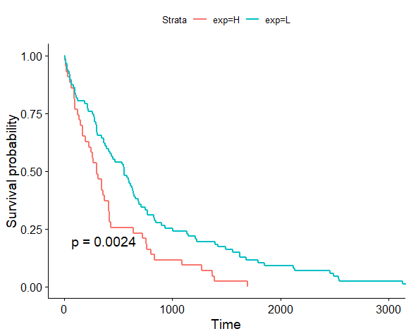
fit <- survfit(Surv(days_to_death, vital_status)~exp, data=df) # 根据表达建模
# 显示P value
surv_pvalue(fit)$pval.txt 
# 画图
ggsurvplot(fit,pval=TRUE)